Automatic differentiation in C++ from scratch
Deep learning frameworks like PyTorch and TensorFlow rely on derivative computation mechanisms to compute the gradient of neural networks. Automatic differentiation is an algorithm that makes the computation of these derivatives easy. In this article, a demonstrative implementation of automatic differentiation will be shown using C++20 and the Eigen library for linear algebra operations.
In a follow-up article, we will train a simple neural network based on the implementation of this article.
How computational graphs work
Computational graphs represent complex calculations as a network of simple operations. Here are their main principles:
- Each node in the graph represents either a variable or an operation
- Edges between nodes show how data flows through the computation
- Each node only depends on its direct inputs
- The graph is evaluated from inputs to outputs (bottom to top)
 Computational graphs are used everywhere because they make easier the computation of derivatives by using automatic differentiation.
Calculating the derivatives
To compute derivatives, we have several options. Let’s see why automatic differentiation is usually preferred:
Numerical Differentiation
To calculate the derivative of a function, we could use numerical differentiation, which relies on the partial derivative definition:
\[\dfrac{\partial}{\partial x_i} f(\textbf{a}) = \lim_{h \to 0} \frac{f(\textbf{a} + h\textbf{e}_i) - f(\textbf{a})}{h}\]Where \(\textbf e_i\) is the unit vector whose \(i\)th component is \(1\) and all the other components are \(0\) Numerical differentiation calculates an approximation of the derivative by letting \(h\) be a small finite number. However, this method has a few drawbacks:
- It introduces numerical imprecision
- It suffers from floating-point rounding errors
- It requires multiple graph evaluations, one for each input variable
A better alternative would be to use automatic differentiation, which does not have these three flaws.
Automatic differentiation
Automatic differentiation has two approaches: forward-mode and reverse-mode. Both computes the exact derivatives up to floating-point precision but with different computational characteristics.
- Forward Mode
- Traverses graph from inputs to outputs
- Calculates derivatives with respect to one input at a time
- Efficient for functions with few inputs and many outputs
- Reverse Mode
- Traverses graph from outputs to inputs
- Calculates derivatives of one output with respect to all inputs in a single pass
- Ideal for functions with many inputs and few outputs (common in deep learning)
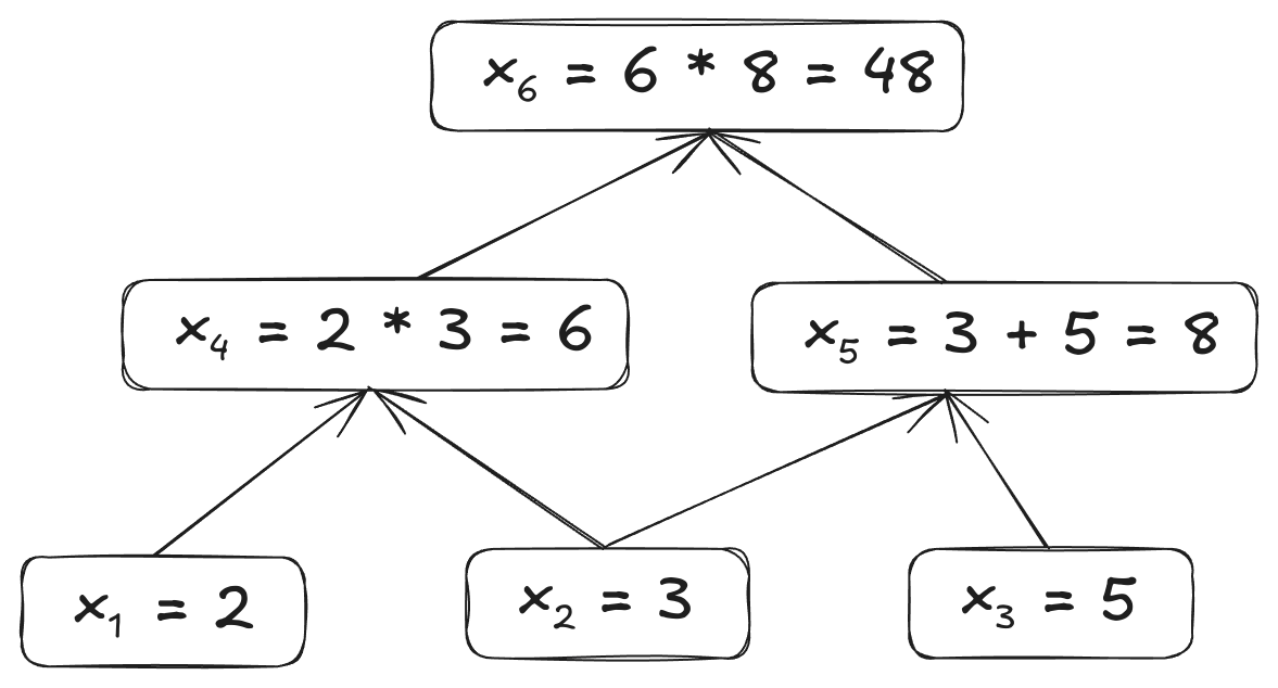
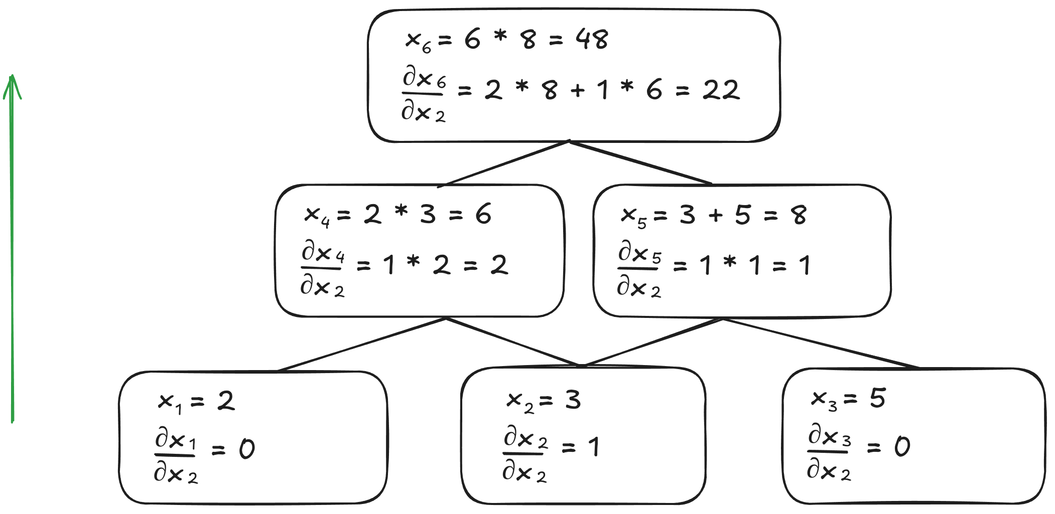 Forward-mode differentiation when calculating \(\frac{dx_6}{dx_2}\)
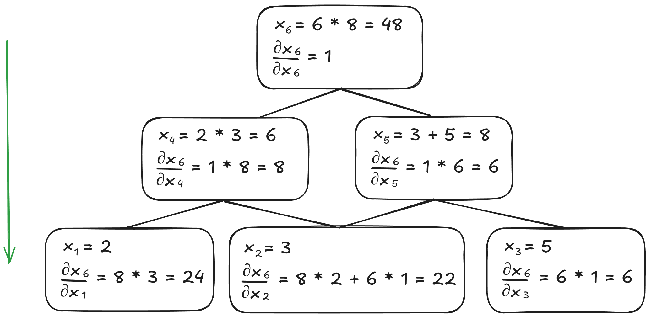 Reverse-mode differentiation when calculating \(\frac{dx_6}{dx_2}\)
These two algorithms can achieve the same result. However, the only difference is the number of times the graph must be traversed. To compute the derivative of all inputs with forward-mode differentiation, the graph would need to be traversed as many times as there are inputs. On the other hand, reverse-mode differentiation only requires the graph to be traversed once to compute the derivative of all the inputs. For our implementation, we will focus on reverse-mode differentiation since it is particularly adapted to deep learning applications where we typically have more inputs than outputs.
A Small Note
The derivative of an input in a graph is the sum of all the paths from that input to the output. This follows from the multivariate chain rule:
\[\frac{dh}{dx_1} = \frac{\partial h}{\partial x_2}\frac{df}{dx_1} + \frac{\partial h}{\partial x_3}\frac{dg}{dx_1}\]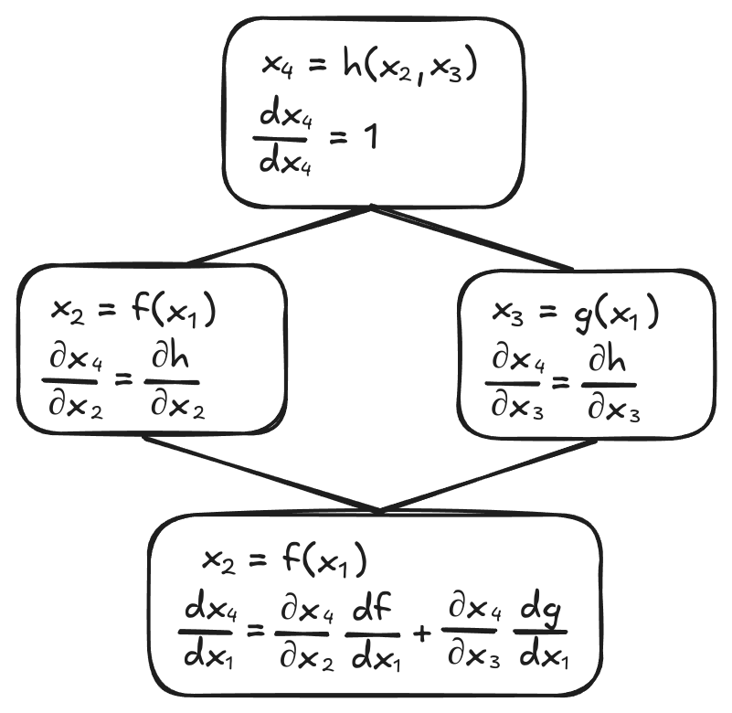
Using matrices
Calculating the derivative of matrices is not as straightforward as with scalars. In this section, I will demonstrate the formulas.
Calculating the derivative of the matrix product
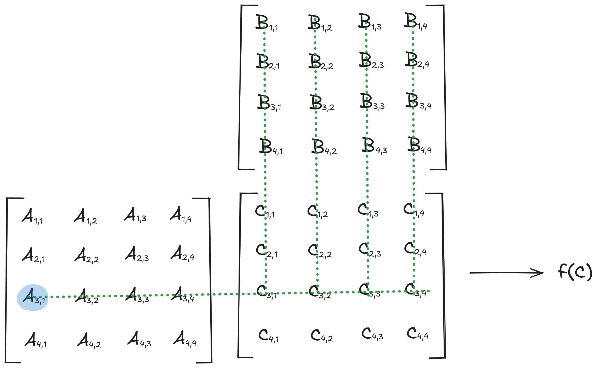
Let \(\textbf C\) be the matrix product of \(\textbf{A} \in \mathbb{R}^{m \times n}\) and \(\textbf{B} \in \mathbb{R}^{n \times p}\)
\[\textbf{C}=\textbf{A}\textbf{B}\]The equation above can also be written with the sigma notation as:
\[\textbf{C}_{i,j}=\sum_{k=1}^n \textbf{A}_{i,k} \textbf{B}_{k,j}\]Therefore, the partial derivative of \(\textbf{C}_{i,j}\) with respect to \(\textbf{A}_{i,k}\) and \(\textbf{B}_{k,j}\) are respectively
\[\frac{\partial \textbf{C}_{i,j}}{\partial \textbf{A}_{i,k}}=\textbf{B}_{k,j}\] \[\frac{\partial \textbf{C}_{i,j}}{\partial \textbf{B}_{k,j}}=\textbf{A}_{i,k}\] \[\text{ For all possible values of } i,j,k\]Now let’s assume the final output \(f(\textbf C)\) is a scalar, then \(\frac{\partial f}{\partial \textbf{C}} \in \mathbb{R}^{m \times n}\) for a function \(f \colon \mathbb{R}^{m \times n} \to \mathbb{R}\).
The partial derivative of \(f\) with respect to \(\textbf{A}_{i,k}\) and \(\textbf{B}_{k,j}\) are then respectively
\[\frac{\partial f}{\partial \textbf{A}_{i,k}} = \sum_{j=1}^{p} \left( \frac{\partial f}{\partial \textbf{C}} \right)_{i,j} \cdot \textbf{B}_{k,j}\] \[\frac{\partial f}{\partial \textbf{B}_{k,j}} = \sum_{i=1}^{m} \left( \frac{\partial f}{\partial \textbf{C}} \right)_{i,j} \cdot \textbf{A}_{i,k}\]As an example:
It can be written in matrix form
\[\frac{\partial f}{\partial \textbf{A}} = \frac{\partial f}{\partial \textbf{C}} \textbf{B}^T\] \[\frac{\partial f}{\partial \textbf{B}} = \textbf{A}^T \frac{\partial f}{\partial \textbf{C}}\]The implementation
We could implement some linear algebra operations ourselves, however, doing this would be too much work for this article. Instead, we are going to use the highly optimized Eigen library. To keep this article short, the implementation will be minimal and thus unoptimized, as you will see later.
Core Design: Expressions
The aim is to build a graph where each node represents a mathematical operation.
This will be represented by the Expr class.
It will be a pure virtual interface, from which every type of expression will inherit.
We will use polymorphism because nodes should be able reference their children without knowing their types at runtime.
expr.hpp
#pragma once
#include <memory>
#include <Eigen/Dense>

template<typename T>
struct Expr
{
Eigen::MatrixX<T> value;
Eigen::MatrixX<T> gradient;
bool requires_gradient = false;

template<typename Derived>
Expr(const Eigen::EigenBase<Derived>& v) : value(v) {}
virtual ~Expr() {}

virtual void backward(const Eigen::Ref<const Eigen::MatrixX<T>>& g)
{
if (requires_gradient) {
    gradient += g;
}
}

void clear_gradient()
{
if (requires_gradient) {
    gradient.resizeLike(value);
    gradient.setZero();
}
}
};

template<typename Derived>
Expr(const Eigen::EigenBase<Derived>&) -> Expr<typename Derived::Scalar>;
The classes derived from Expr will represent the result of an operation.
They will keep track of their inputs and override the inherited virtual backward function that computes and propagates the gradient.
The clear_gradient method will set the gradient to 0.
Note that the backward method adds the gradient coming from different paths, as mentioned in the note previously.
The purpose of the requires_gradient boolean is to avoid storing the gradient of a node when it is not necessary.
The expression at the bottom is a deduction guide of C++20, it helps for CTAD.
The matrix class
The Matrix class will represent a dense matrix for the user.
It will manage the expression graph by storing a shared pointer to an Expr class that will hold the actual data.
matrix.hpp
template<typename T>
class Matrix
{
public:
Matrix(size_t rows, size_t cols)
: expr_{ std::make_shared<Expr<T>>(Eigen::MatrixX<T>(rows, cols)) }
{
}

Matrix(const std::initializer_list<std::initializer_list<T>>& list)
: expr_{ std::make_shared<Expr<T>>(Eigen::MatrixX<T>(list)) }
{
}

template<typename Derived>
explicit Matrix(const Eigen::EigenBase<Derived>& matrix)
: expr_{ std::make_shared<Expr<T>>(matrix) }
{
}

const auto& eigen() const { return expr_->value; }

private:
template<template<typename> class ExprLike>
Matrix(std::shared_ptr<ExprLike<T>> expr)
: expr_{ std::dynamic_pointer_cast<Expr<T>>(std::move(expr)) }
{
}

std::shared_ptr<Expr<T>> expr_;
};

template<typename Derived>
Matrix(const Eigen::DenseBase<Derived>&) -> Matrix<typename Derived::Scalar>;

template<typename T>
std::ostream& operator<<(std::ostream& os, const Matrix<T>& matrix)
{
return os << matrix.eigen();
}
This wrapper uses shared pointers to manage the lifetime of expressions and allows nodes to remain even after their creating matrices goes out of scope. We define the constructors and the ostream operator. The private constructor will be used when creating new expressions, it will avoid repeating the shared pointer cast. Let’s now implement some simple utility functions
matrix.hpp
template<typename T>
class Matrix
{
public:
/* ... */

size_t rows() const { return expr_->value.rows(); }
size_t cols() const { return expr_->value.cols(); }
size_t size() const { return expr_->value.size(); }

void resize(size_t rows, size_t cols)
{
expr_->value.resize(rows, cols);
}

const auto& eigen() const { return expr_->value; }

T& operator()(size_t i, size_t j) { return expr_->value(i, j); }
const T& operator()(size_t i, size_t j) const { return expr_->value(i, j); }

bool operator==(const Matrix& other) const { return expr_->value == other.expr_->value; }
template<typename Derived>
bool operator==(const Eigen::MatrixBase<Derived>& other) const { return expr_->value == other; }

bool is_approx(const Matrix& other) { return expr_->value.isApprox(other.expr_->value); }
template<typename Derived>
bool is_approx(const Eigen::MatrixBase<Derived>& other) { return expr_->value.isApprox(other); }

/* ... */
};
Operations
Let’s implement some base classes that will represent the derived expressions. They can be of the different types:
UnaryExpr: expressions that have one matrix as inputBinaryExpr: expressions that have two matrices as inputsScalarExpr: expressions that have one matrix and one constant scalar as inputs
expr.hpp
/* ... */

template<typename T>
struct UnaryExpr : Expr<T>
{
std::shared_ptr<Expr<T>> input;

template<typename Derived>
UnaryExpr(const Eigen::EigenBase<Derived>& v, std::shared_ptr<Expr<T>> i)
: Expr<T>(v), input(i) {}
};


template<typename T>
struct BinaryExpr : Expr<T>
{
std::shared_ptr<Expr<T>> left;
std::shared_ptr<Expr<T>> right;

template<typename Derived>
BinaryExpr(const Eigen::EigenBase<Derived>& v, const std::shared_ptr<Expr<T>>& l, const std::shared_ptr<Expr<T>>& r)
: Expr<T>(v), left(l), right(r) {}
};


template<typename T>
struct ScalarExpr : UnaryExpr<T>
{
T scalar;

template<typename Derived>
ScalarExpr(const Eigen::EigenBase<Derived>& v, std::shared_ptr<Expr<T>> i, T s)
: UnaryExpr<T>(v, i), scalar(s) {}
};
Here is how we implement binary operations like matrix addition and multiplication:
expr.hpp
/* ... */

template<typename T>
struct AddExpr : BinaryExpr<T>
{
AddExpr(const std::shared_ptr<Expr<T>>& l, const std::shared_ptr<Expr<T>>& r)
: BinaryExpr<T>(l->value + r->value, l, r)
{
}

void backward(const Eigen::Ref<const Eigen::MatrixX<T>>& g) override
{
BinaryExpr<T>::backward(g);
this->left->backward(g);
this->right->backward(g);
}
};

template<typename T>
struct MultiplyExpr : BinaryExpr<T>
{
MultiplyExpr(const std::shared_ptr<Expr<T>>& l, const std::shared_ptr<Expr<T>>& r)
: BinaryExpr<T>(l->value * r->value, l, r)
{
}

void backward(const Eigen::Ref<const Eigen::MatrixX<T>>& g) override
{
BinaryExpr<T>::backward(g);
this->left->backward(g * this->right->value.transpose());
this->right->backward(this->left->value.transpose() * g);
}
};
Now a ScalarExpr:
expr.hpp
template<typename T>
struct MultiplyScalarExpr : ScalarExpr<T>
{
MultiplyScalarExpr(const std::shared_ptr<Expr<T>>& input, T scalar)
: ScalarExpr<T>(input->value * scalar, input, scalar)
{
}

void backward(const Eigen::Ref<const Eigen::MatrixX<T>>& g) override
{
ScalarExpr<T>::backward(g);
this->input->backward(g * this->scalar);
}
};
The implementation of SubtractExpr</var>, <var>DivideScalarExpr</var>, and <var>TransposeExpr are not shown here as they are really similar to the ones above.
Here are some more complex operations, like the ReLU activation function and the matrix norm.
CwiseMaxExpr is just a fancy name for the ReLU function. Or \(f(x)=\max\{0, x\}\).
expr.hpp
/* ... */

template<typename T>
struct NormExpr : UnaryExpr<T>
{
NormExpr(const std::shared_ptr<Expr<T>>& input)
: UnaryExpr<T>(Eigen::MatrixX<T>{{ input->value.norm() }}, input)
{
}

void backward(const Eigen::Ref<const Eigen::MatrixX<T>>& g) override
{
UnaryExpr<T>::backward(g);
this->input->backward(g.value() / this->value.value() * this->input->value);
}
};


template<typename T>
struct CwiseMaxExpr : UnaryExpr<T>
{
CwiseMaxExpr(const std::shared_ptr<Expr<T>>& input)
: UnaryExpr<T>(input->value.cwiseMax(0), input)
{
}

void backward(const Eigen::Ref<const Eigen::MatrixX<T>>& g) override
{
UnaryExpr<T>::backward(g);
this->input->backward(g.array() * (this->input->value.array() > 0.0).template cast<T>());
}
};
Back to the matrix class
To use the operations we just implemented, we need to implement the respective operations in the Matrix class
matrix.hpp
template<typename T>
class Matrix
{
public:
/* ... */
Matrix operator+(const Matrix& other) const
{
return std::make_shared<AddExpr<T>>(expr_, other.expr_);
}

Matrix operator*(const Matrix& other) const
{
return std::make_shared<MultiplyExpr<T>>(expr_, other.expr_);
}

Matrix transpose() const
{
return std::make_shared<TransposeExpr<T>>(expr_);
}

Matrix norm() const
{
return std::make_shared<NormExpr<T>>(expr_);
}

Matrix cwise_max() const
{
return std::make_shared<CwiseMaxExpr<T>>(expr_);
}
};
This is a lot of repeated code, as they all return an expression of their respective operation. I have just included here the essential ones The last thing we need to implement are some utility functions related to the computation of gradients
matrix.hpp
template<typename T>
class Matrix
{
public:
/* ... */

void backward() const
{
if (expr_->value.rows() != 1 || expr_->value.cols() != 1) {
    throw std::logic_error{ "backward can only be called on 1x1 matrices (scalars)" };
}
expr_->backward(Eigen::MatrixX<T>{{1}});
}

const Eigen::MatrixX<T>& gradient() const
{
return expr_->gradient;
}

bool& requires_gradient() { return expr_->requires_gradient; }

bool requires_gradient() const { return expr_->requires_gradient; }

Matrix& set_requires_gradient()
{
expr_->requires_gradient = true;
expr_->clear_gradient();
return *this;
}

Matrix& clear_gradient()
{
expr_->clear_gradient();
return *this;
}
};
Usage and Testing
Let’s do some tests with the Google test library to check that our classes work correctly.
test_matrix.cpp
#include <gtest/gtest.h>
#include "matrix.hpp"

TEST(test_matrix, handles_matrix_gradient)
{
Matrix<float> a = { {1, 2}, {3, 4} };
Matrix<float> b = { {5, 6}, {7, 8} };
a.set_requires_gradient();
b.set_requires_gradient();

auto c = a - b;
auto d = a + b;

auto e = c * d;

auto f = e.sum();

a.clear_gradient();
b.clear_gradient();
f.backward();

EXPECT_EQ(a.gradient(), (Matrix<float>{{6, 14}, { 6, 14 }}));
EXPECT_EQ(b.gradient(), (Matrix<float>{{-22, -30}, { -22, -30 }}));

auto g = e.mean();

a.clear_gradient();
g.backward();

EXPECT_EQ(g, (Matrix<float>{{-72}}));
EXPECT_EQ(a.gradient(), (Matrix<float>{{1.5, 3.5}, { 1.5, 3.5 }}));

auto h = (d + c * 2.2).cwise_max().norm();
auto i = h.cwise_max().norm();

a.clear_gradient();
b.clear_gradient();
h.backward();

EXPECT_TRUE(h.is_approx(Matrix<float>{{3.4176}}));
EXPECT_TRUE(a.gradient().isApprox(Eigen::MatrixXf{{0, 0}, { 1.12359, 2.99625 }}));
EXPECT_TRUE(b.gradient().isApprox(Eigen::MatrixXf{{0, 0}, { -0.421348, -1.12359 }}));
}
Future improvements
The implementation works, but it could be improved by
- Eliminating temporary objects using Eigen’s expression templates (as every current operation creates a temporary)
- Implementing memory pooling for expression nodes
- Adding support for more operations and optimizations
In the second part of this article, we will use this implementation to train a neural network!
Conclusion
This implementation is just a demonstration, but it still shows a fully-working automatic differentiation algorithm.